States across the U.S. vary widely in geographic size and distance from one another, which can make mapping tricky when following data visualization best practices. These tips will help you choose the best approach for your map.
Before we begin, let's review our options for the right map type.
There are a handful of basic maps that you can choose from including:
Scroll through the workbook tabs below to view the advantages of different maps.
For the tips below, we are going to stick with choropleth maps (filled or shaded maps) as they are the most popular type of map visualization.
Hex-tile maps are highly recommended by data viz experts because they are a solid workaround for a common problem in visualizing choropleth data equally - especially in respect to smaller New England states and Alaska. The fundamental issue we face in mapping the United States is that the size and distance of our states and territories are playing a role in the visualization when they should not. The workaround is to make the land-size equal so the color of the measures are better represented. This is a great use case for hex-tile maps!
Check out Zen Master Kevin Flerlage's (The Flerlage Twins) blog post on hex-tile maps.
Download the X and Y Coordinates and a hexagon to use for your shape.
(Need more help? Click here for how to add a custom shape.)
Bonus:
United Kingdom hex-tile map by James Smith (Sports Chord)
India hex-tile map by Satish Ramakrishna (Revizited)
A hex-tile map is created by generating our own X and Y axes and plotting our placement of the states and territories with these X, Y coordinates. Hexagons are used as the shape to better capture the "corners" of our country. Squares or circles will work, but they don't look as lovely. Also, notice how Alaska, Hawaii, and Washington, D.C. are separate? We can also easily represent Puerto Rico and other US territories data in the lower part of map as well.
Not ready to embrace hex-tile maps yet? No worries! We can still choose a traditional map view.
For these examples, we will be working with Tableau's handy Obesity data source located in the Regional Sample Workbook with a few tweaks. (Download it here.)
Below is a choropleth map of the United States including Alaska and Hawaii.
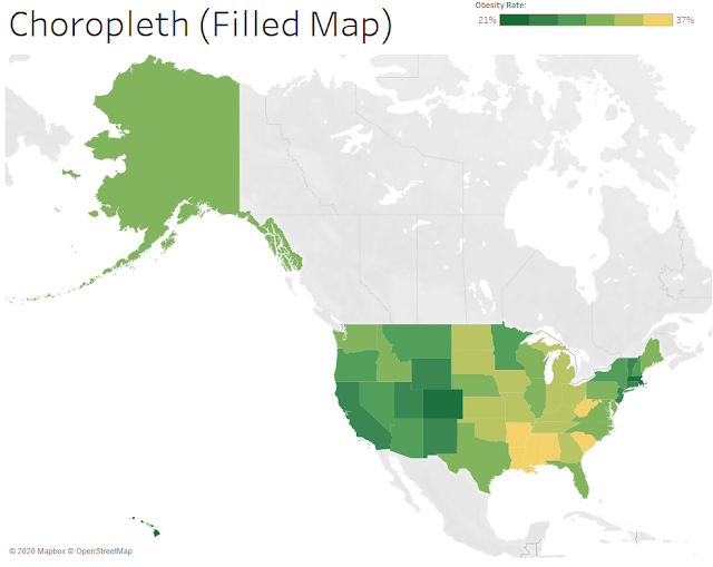
We can easily see Alaska, as well as the other larger states, but what about Connecticut or Rhode Island? Due to their small geographic size, they are muffled in this representation. The best way to fix this is to create separate and rescaled maps to standardize the different sizes and distances from the other states.
If your data is continuously updated or you use a parameter to toggle measures, this is not a wise decision.
However, if the min and max value of the data is static, and you are not using a parameter to switch measures on color, filtering out these states can be a good idea.
The reason for this caveat is that we have to lock the color legend in the Advanced settings to continue to represent the correct color range. This means we include a Start and End value for the color range. Since these values have to be hardcoded, it typically only makes sense for one measure. Furthermore, if your data is frequently updated, this step will need to be done manually any time there is an update to the min or max value. This is quite cumbersome.
Let's review an example:
Check out Alaska's Obesity percentage value and color. It is 31% and green. (Remember this.)
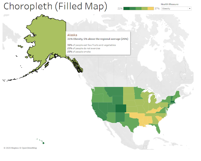
Now duplicate this worksheet and then filter to only include Alaska.
Remember above how Alaska's value of 31% Obesity was green?
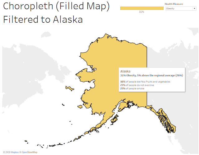
Oh no! Alaska is now yellow instead of green. This is because when we filter to only include Alaska, we lose the color gradient and just have one data point for the range. If we add this filtered map of Alaska alongside the contiguous United States, the color will not be representative of the value range and our visualization will be wrong.
To fix this, we manually lock the Start and End value of the Color range to the min value and max value of our single measure of Obesity, which is 21% and 37%, respectively.
Marks Box > Color > Edit Colors > Advanced
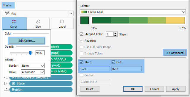
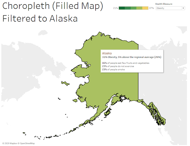
Fixed it!
Note that we hardcoded our Start and End values. If we use a parameter to toggle the measure color, the min and max will not be dynamic to the ranges of separate measures.
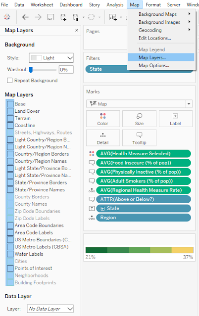
To make the map nice and tidy, we remove all map layers. This will give us a pleasant white background and allow transparency for the maps. This is a must-have for good floating placement in Step 5. Go to Map > Map Layers. Then unselect all options on the left.
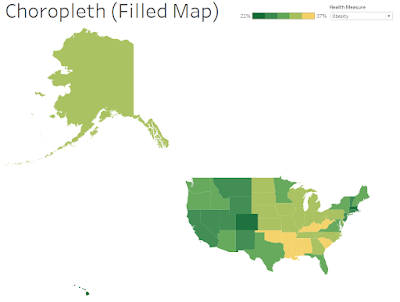
In this example we will create a separate and rescaled map for Alaska and Hawaii to float on a dashboard with the contiguous United States.
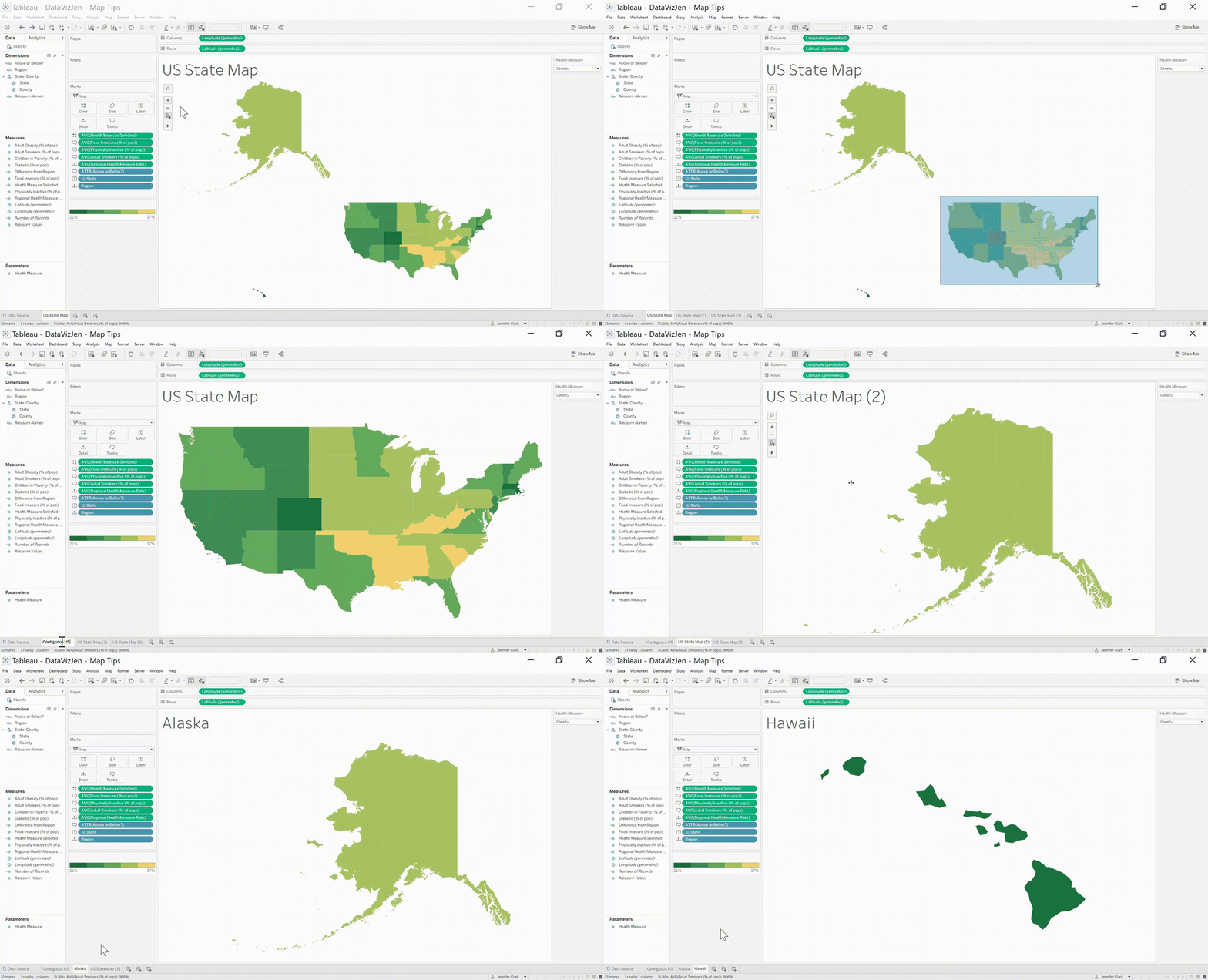
The first step is to duplicate the map two times.
Next either zoom into the contiguous United States or, if you have static data and only one measure on color, filter out Alaska and Hawaii.
After that, unselect all of the Map Options so users cannot adjust your map. Or better yet, accidentally zoom in when they are using a mouse to scroll down the dashboard - which is a common frustration many viewers experience.

Watch a demonstration of how to separate and rescale:
Step 5: Create a dashboard with all maps together.
Recall in Step 3 when we removed all map layers? This is where it pays off! If you missed this step, you'll want to do it now. Removing the map layers will provide us with a transparent worksheet to float on the dashboard. This gives us a lot more options on placement.
Happy vizzing! 💗



Have a question or just want to say hi?
I'd love to hear from you.